
29 Sep Digital Signal Transmission
29/09/2021
Foreword: We continue to celebrate the month of electrical engineering, within the cycle of the 40th anniversary of Im3.
Although this news and its continuation refer to the transmission of digital signals through electrical and optical cables, the concepts and laws referred to constitute the conceptual basis for the development of communication projects by means of electromagnetic waves in any medium, including fields of maximum interest to Im3 such as: communications in substations and digital networks, LiDAR technology, carrier wave, microwave, geo-radar (GPR), 5G communications, Wi-Fi, IoT, FTTH deployment or implementation of smart metering systems. And even the behavior of lines and earth meshes against atmospheric discharges.
The propagation of an electrical signal in the form of an electromagnetic (EM) wave through conductive cables travels at a speed of approximately:
• 80-90% the speed of light in vacuum (c)
• 2.4-2.7 x 10⁸ m / s
• 24-27 cm / ns
On the other hand, every electrical pulse transmitted in a conducting medium can be represented as the sum of its sinusoidal components of different frequencies (Fourier’s theorem).
And due to the impedance of the cable (mainly its inductance), the different frequency components of electrical signals travel at different speeds and experience different attenuations.
Attenuation is the gradual reduction in the intensity of the wave through the medium, which in sinusoids that move linearly consists of the decrease in the amplitude of the wave between the emission and its receiver.
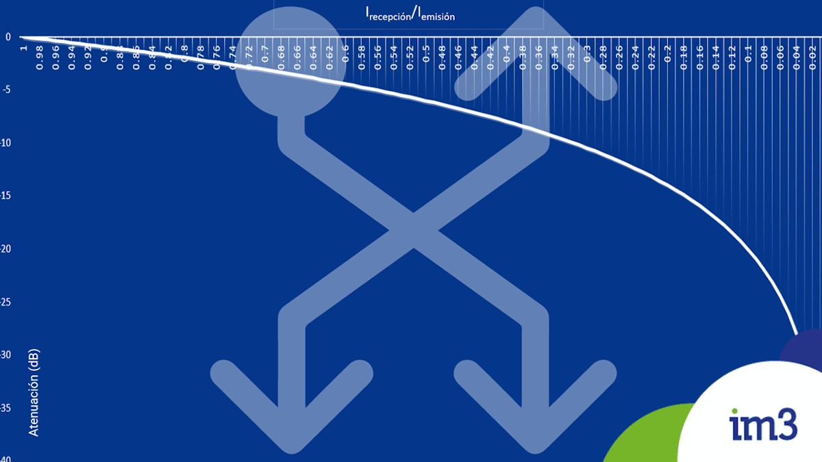
Power attenuation α is calculated in decibels (dB) as α = 10 log (P_reception / P_emission)
= 10 log (R*I_ reception^2 / R*I_ emission ^2) = 10 log ((I_reception / I_emission)^2)
= 2*10 log (I_reception / I_emission) = 20*log (I_reception / I_emission)
The attenuation in the transmission of a signal usually oscillates between 0dB (without the presence of attenuation) and -40dB (see graphic in the image of the news). This range or system gain can be as wide as 120dB depending on the technology. For reference:
• An attenuation of -6.02 dB corresponds to a reduction of half (1/2) the amplitude of the signal (respectively a quarter of the power).
• And an attenuation of -9.54 dB, represents a reduction of one third (1/3) of its amplitude.
On the other hand, the fact that the waves travel at different speeds means that they reach the receiver with time lags, which increase in direct proportion to the length of the conductor (distance between emitter and receiver).
This ‘low pass’ effect causes both the rising and falling ends of the pulse to deviate in time, a phenomenon known as dispersion (frequency-dependent phase velocity) and which, together with interference, could cause jitter (which is the difficulty to recover the clock from a signal)
Since the exposed phenomena are limiting factors for the integrity of the signal reception, they will condition the maximum length of the conductor (L) for each transmission frequency (or channel bandwidth). And, if we include external noise in the equation, therefore, it limits your channel transmission capacity.
Recall that, according to Shannon’s theorem, the capacity of an ideal channel in bits/s is equal to C = B * log2 (1 + S / N), where B is the bandwidth of the channel in Hz, S is the power of the useful signal in W and N the power of the noise present in the channel in W. This means that, if the medium is dedicated, there would be no limit to the bandwidth by the medium. But this is not the case, even in the absence of attenuation.
As a ‘rule of thumb’, for traditional cabling, we can say that the transmission of data, in baseband, through the channel will be technically feasible when the length of the line is reduced compared to the wavelength of the signal ( λ), approximately L <λ/100.
For example, for a copper conductor of L = 100 meters, the maximum data transmission frequency would be that in which λ = 100/100 = 1m, which for a propagation speed of 2.55 x 10⁸ would correspond to an fmax ≈ 2.55 x 10⁸ / 1 = 255 x 106 = 255 MHz.
To overcome this rate limitation, the materials selected for the construction of the wiring evolve to improve their standards. In simple terms, the new standards seek among other things: to eliminate dispersion, by building a medium with a constant phase velocity, up to at least the order of magnitude of the bandwidth of the bit rate (or baseband).
The above frequency corresponds to a period of T = 1 / 255M Hz = 3.9215 x 10⁹ sec = 3.9215 x 10⁶ ms = 3.9215 x 10³ μs = 3.9215 ns (equivalent to the time it takes for light to travel 1.17 meters in vacuum)
Currently, for Ethernet networks with twisted pair cables, the higher technology categories have the following bandwidths:
• Cat7 (600 MHz) category F according to ISO EN 50173
• Cat7A (1000 MHz) category FA according to ISO EN 50173
• Cat 8 / 8.1 (2000 MHz) ISO / IEC 11801-1: 2017
• Cat 8.2 (2000 MHz) ISO / IEC 11801-1: 2017
Important: The above categories can be used with guarantees of signal integrity as long as the cable lengths are less than 100 meters.
References:
Signal Integrity vs. Transmission Rate and Cable Length for Rs-485 Transceivers, Application Report SLLA375 – September 2017, Texas Instruments
Signals, The Science of Telecommunications, John R. Pierce and A. Michael Noll, Editorial Reverté, S.A., 1995